B-tree highlights from the Database internals book
Most of the mutable storage structures use an in-place update mechanism. During insert, delete, or update operations, data records are updated directly in their locations in the target file.
B-Trees combine ideas: increase node fanout, and reduce tree height, the number of node pointers, and the frequency of balancing operations.
B-Trees can be thought of as a vast catalog room in the library: you first have to pick the correct cabinet, then the correct shelf in that cabinet, then the correct drawer on the shelf, and then browse through the cards in the drawer to find the one you’re searching for. Similarly, a B-Tree builds a hierarchy that helps to navigate and locate the searched items quickly.
B-Trees build upon the foundation of balanced search trees and are different in that they have higher fanout (have more child nodes) and smaller height.
B-Trees are sorted: keys inside the B-Tree nodes are stored in order
This also implies that lookups in B-Trees have logarithmic complexity
Using B-Trees, we can efficiently execute both point and range queries. Point queries, expressed by the equality (=) predicate in most query languages, locate a single item. On the other hand, range queries, expressed by comparison (<, >, ≤, and ≥) predicates, are used to query multiple data items in order.
B-Tree Hierarchy
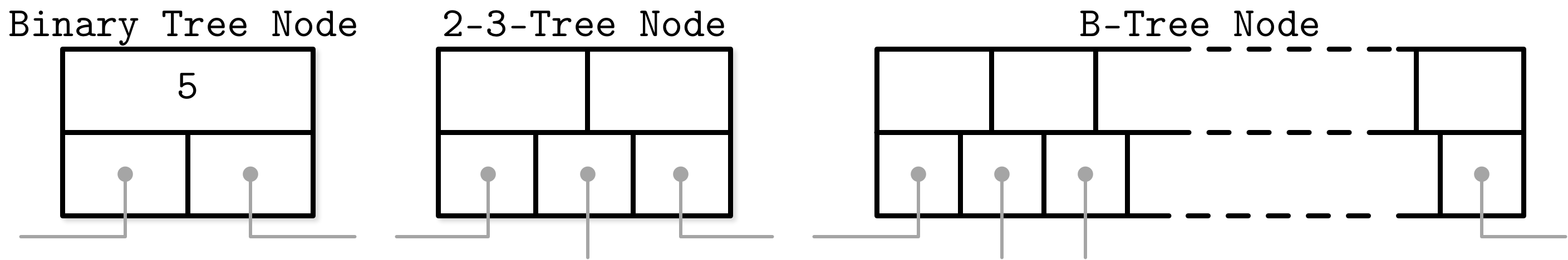
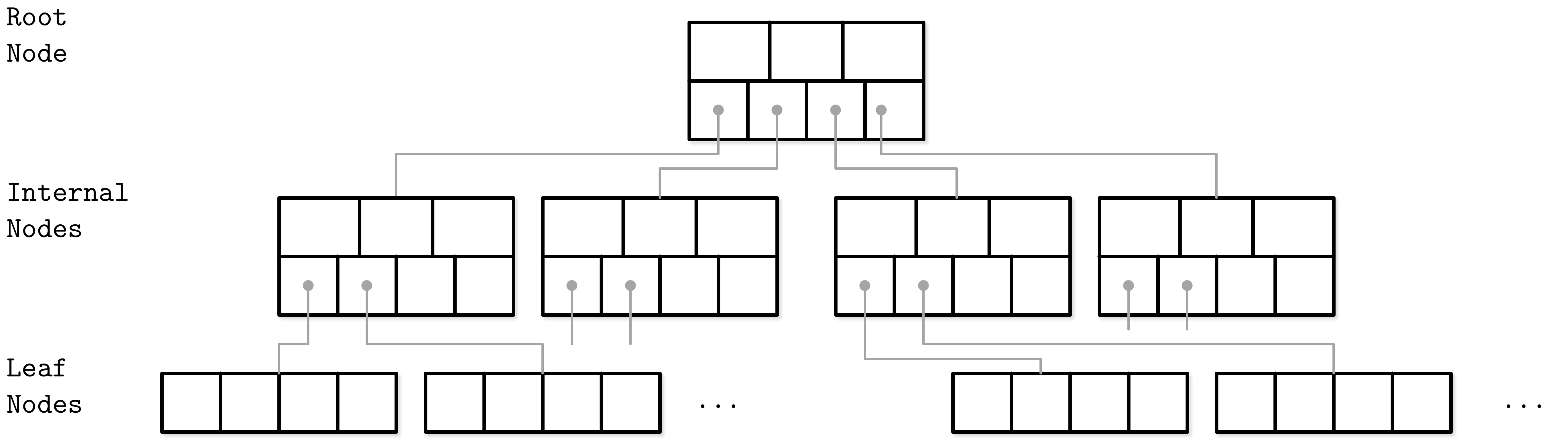
B-Trees consist of multiple nodes. Each node holds up to N keys and N + 1 pointers to the child nodes. These nodes are logically grouped into three groups:
Root node This has no parents and is the top of the tree.
Leaf nodes These are the bottom layer nodes that have no child nodes.
Internal nodes These are all other nodes, connecting root with leaves. There is usually more than one level of internal nodes.
Since B-Trees are a page organization technique (i.e., they are used to organize and navigate fixed-size pages), we often use terms node and page interchangeably.
The relation between the node capacity and the number of keys it actually holds is called occupancy.
B-Trees are characterized by their fanout: the number of keys stored in each node. Higher fanout helps to amortize the cost of structural changes required to keep the tree balanced and to reduce the number of seeks by storing keys and pointers to child nodes in a single block or multiple consecutive blocks. Balancing operations (namely, splits and merges) are triggered when the nodes are full or nearly empty.
$B^+$- tree
B-Trees allow storing values on any level: in root, internal, and leaf nodes. B+-Trees store values only in leaf nodes. Internal nodes store only separator keys used to guide the search algorithm to the associated value stored on the leaf level.
Since values in B+-Trees are stored only on the leaf level, all operations (inserting, updating, removing, and retrieving data records) affect only leaf nodes and propagate to higher levels only during splits and merges.
B+-Trees became widespread, and we refer to them as B-Trees, similar to other literature the subject. For example, in GRAEFE11 B+-Trees are referred to as a default design, and MySQL InnoDB refers to its B+-Tree implementation as B-tree.
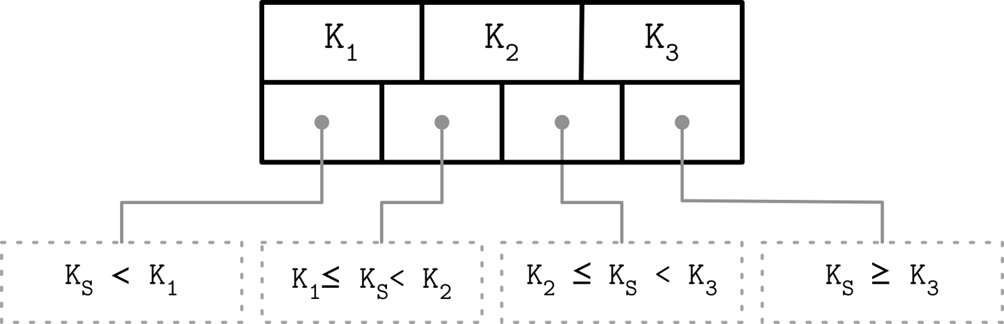
Separator Keys Keys stored in B-Tree nodes are called index entries, separator keys, or divider cells. They split the tree into subtrees (also called branches or subranges), holding corresponding key ranges. Keys are stored in sorted order to allow binary search. A subtree is found by locating a key and following a corresponding pointer from the higher to the lower level.
What sets B-Trees apart is that, rather than being built from top to bottom (as binary search trees), they’re constructed the other way around—from bottom to top. The number of leaf nodes grows, which increases the number of internal nodes and tree height.
Since B-Trees reserve extra space inside nodes for future insertions and updates, tree storage utilization can get as low as 50%, but is usually considerably higher. Higher occupancy does not influence B-Tree performance negatively.
B-Tree Lookup Complexity
B-Tree lookup complexity can be viewed from two standpoints: the number of block transfers and the number of comparisons done during the lookup.
In terms of number of transfers, the logarithm base is N (number of keys per node). There are N times more nodes on each new level, and following a child pointer reduces the search space by the factor of N. During lookup, at most logN M (where M is a total number of items in the B-Tree) pages are addressed to find a searched key. The number of child pointers that have to be followed on the root-to-leaf pass is also equal to the number of levels, in other words, the height h of the tree.
B-Tree Lookup Algorithm
To find an item in a B-Tree, we have to perform a single traversal from root to leaf
Finding an exact match is used for point queries, updates, and deletions; finding its predecessor is useful for range scans and inserts.
The algorithm starts from the root and performs a binary search, comparing the searched key with the keys stored in the root node until it finds the first separator key that is greater than the searched value. This locates a searched subtree. As we’ve discussed previously, index keys split the tree into subtrees with boundaries between two neighboring keys. As soon as we find the subtree, we follow the pointer that corresponds to it and continue the same search process (locate the separator key, follow the pointer) until we reach a target leaf node, where we either find the searched key or conclude it is not present by locating its predecessor.
During the point query, the search is done after finding or failing to find the searched key. During the range scan, iteration starts from the closest found key-value pair and continues by following sibling pointers until the end of the range is reached or the range predicate is exhausted.
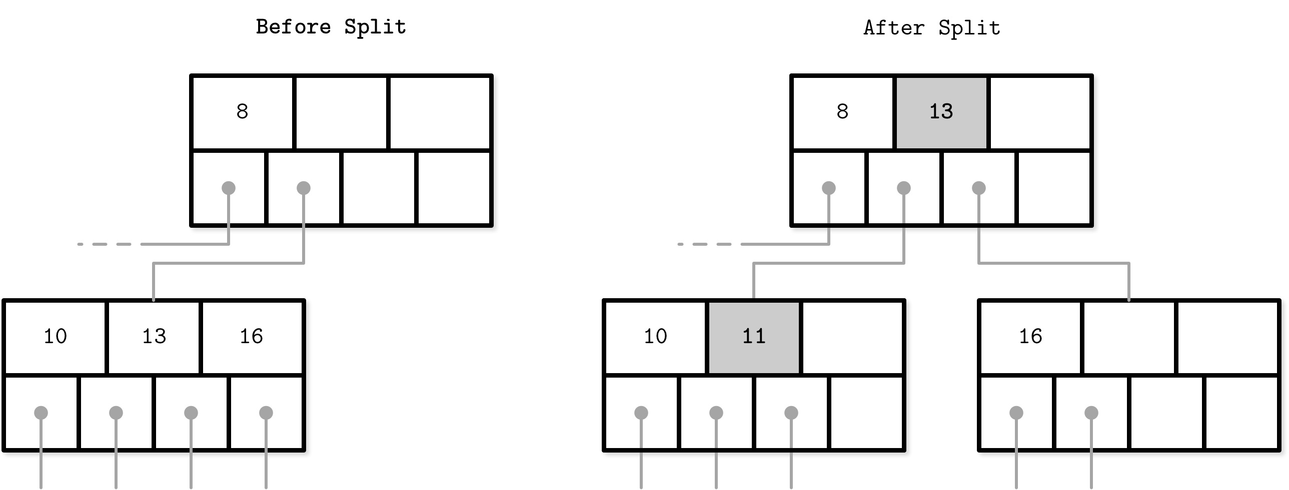
B-Tree Node Splits
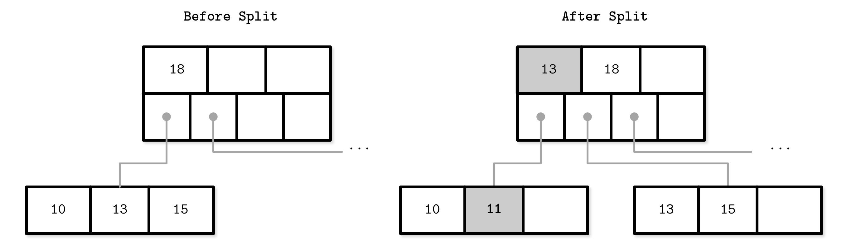
Splits are done by allocating the new node, transferring half the elements from the splitting node to it, and adding its first key and pointer to the parent node. In this case, we say that the key is promoted. The index at which the split is performed is called the split point (also called the midpoint). All elements after the split point (including split point in the case of leaf node split) are transferred to the newly created sibling node, and the rest of the elements remain in the splitting node.
B-Tree Node Merges
Deletions are done by first locating the target leaf. When the leaf is located, the key and the value associated with it are removed.
If neighboring nodes have too few values (i.e., their occupancy falls under a threshold), the sibling nodes are merged. This situation is called underflow. BAYER72 describes two underflow scenarios: if two adjacent nodes have a common parent and their contents fit into a single node, their contents should be merged (concatenated); if their contents do not fit into a single node, keys are redistributed between them to restore balance (see “Rebalancing”).
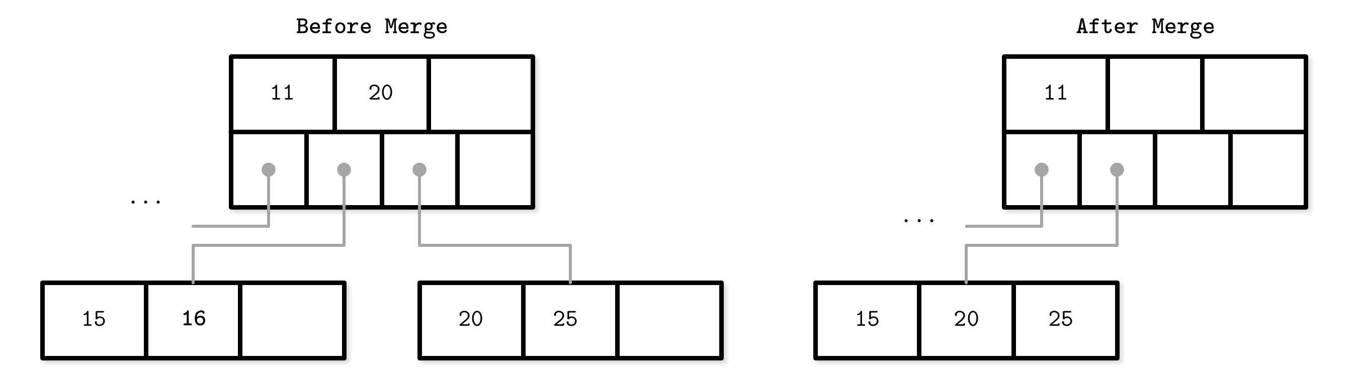
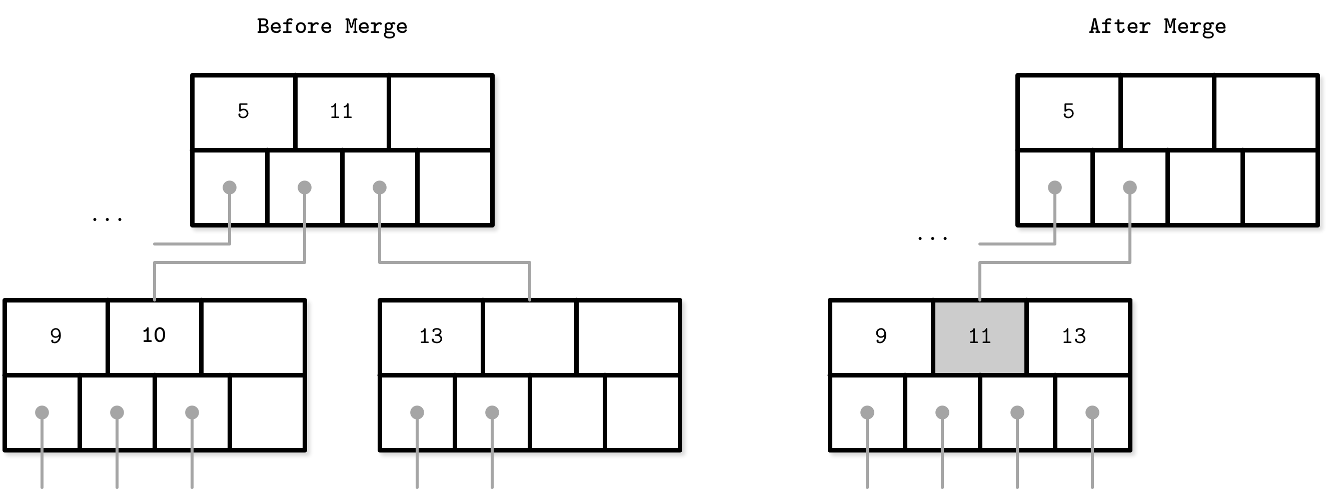
To summarize, node merges are done in three steps, assuming the element is already removed:
- Copy all elements from the right node to the left one.
- Remove the right node pointer from the parent (or demote it in the case of a nonleaf merge).
- Remove the right node.
#books #wip #notes